

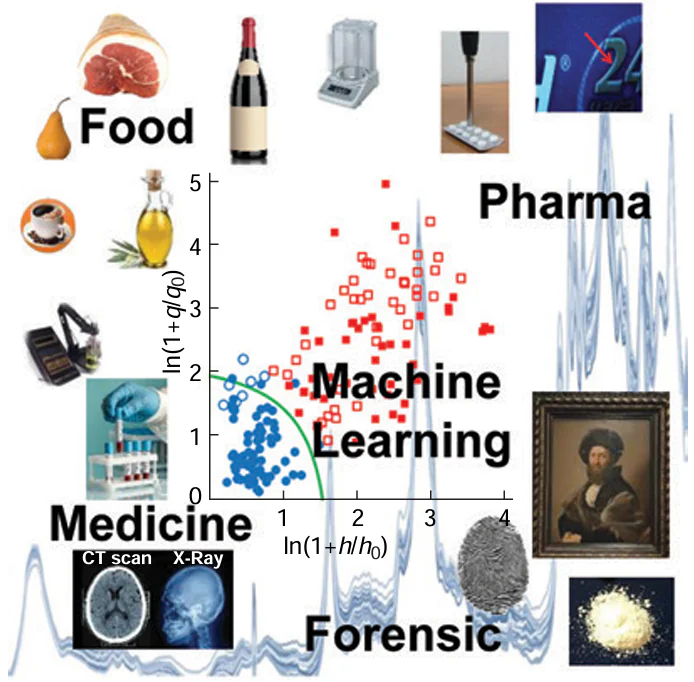
Keywords
Abstract
Non-targeted qualitative analysis has two aspects: instrumental, which involves collection of experimental data needed to solve a given problem, and mathematical, which involves analysis of these data to extract useful information and make reliable decisions. This review is devoted to the latter aspect, namely the general problems of chemometrics and machine learning, which are often incorrectly called artificial intelligence. Various problem formulations are considered, including discrimination and authentication; classification methods (binary, multi-class, or one-class); and types of made decisions (deterministic and probabilistic, soft and hard). Particular attention is given to analytical figures of merit such as sensitivity, specificity, and selectivity and how these characteristics are used for model optimization and validation. The concept of a cumulative analytical signal is also presented, and the prospects for its application in qualitative analysis are discussed.
The bibliography includes 162 references.
1. Introduction
Among numerous analytical chemistry methods, qualitative analysis occupies a special, though not the most prestigious, place. It is responsible for the behind-the-scenes and often nasty work in forensic and customs expertise, medical pathology, food chemistry, and so on. However, unlike its successful ‘big brother’, quantitative analysis, this Cinderella lacks a rich array of luxurious accessories and adornments such as analysis of uncertainties, limits of detection and quantification, and so on. For example, it is well known what is the selectivity in quantitative analysis; there is a definition and methods for calculation. Meanwhile, until recently, there was nothing of the sort in qualitative analysis. Moreover, the International Union of Pure and Applied Chemistry (IUPAC) has not invented a proper definition for qualitative analysis. Officially, the old definition, adopted back in 1995, is still in effect: ‘analysis in which substances are identified or classified on the basis of their chemical or physical properties such as chemical reactivity, solubility, molecular weight, melting point, radiative properties (emission, absorption), mass spectra, nuclear half-life, etc’.[1] According to the traditional understanding, qualitative analysis establishes the presence of particular elements/chemical compounds/functional groups in the analyte sample by means of qualitative test reactions.
However, the scope and methods of qualitative analysis have now markedly expanded beyond the identification of single chemical compounds.[2] Currently, the main trend is non-targeted analysis,[3-5] which focuses not on particular substances, but on analysis of those chemical and physical properties of a sample that make it similar to or distinct from the target sample. In addition, it was proposed to simplify the definition of qualitative analysis,[6] to make it ‘classification according to specified criteria’; however, this minor revolution did not gain support within IUPAC.
Nevertheless, classification is an important and integral part of qualitative analysis. Machine learning and chemometrics offer a wide range of such methods.
Recent reviews address various aspects of the use of classification methods. For example a review by Strani et al.[7] is devoted to a strategy called one-class classification. Issues related to validation of screening methods in the context of qualitative analysis are considered in a review by Cuadros et al.[8] More specific classification issues related to application of experimental data gained using various analytical platforms are discussed in reviews on classification in vibrational spectroscopy[9] and in laser-induced breakdown spectroscopy (LIBS).[10]
The present review focuses not so much on specific methods as on their general characteristics, such as the way of presenting the results (binary or non-binary classification), the purpose of the method (single-class or multi-class one), and, of course, on the methods used to evaluate the quality of the results. In addition, the concept of a cumulative analytical signal is presented, and the prospects for its application are discussed.
To choose an appropriate method, it is necessary, first, to understand what is known and what question needs to be answered. Some typical scenarios in qualitative analysis are considered below.
Identification answers the question: what is it? The answer usually comes from comparison of a certain set of features, e.g., a spectrum or a chromatogram, with another similar set corresponding to a known instance. In practice, this is reduced to searching through known compounds stored in a library. Examples are identification using libraries of mass spectra[11-13] or Raman spectra.[14] This area is extensively addressed by Russian scientists;[15] hence, we will not examine it in detail.
Clusterization investigates a set of similar objects in order to understand to what extent they are uniform and whether they are subdivided into clusters or groups. This approach is called unsupervised classification, since information on the class to which the instances belong is either missing or not used in the modelling. An example of this approach is the analysis of Spanish wine samples using two-dimensional HPLC with fluorescence detection.[16] In essence, clusterization is an exploratory analysis technique used in various fields of analytical chemistry; therefore, it is also excluded from the scope of this review.
Discrimination determines to which of dedicated groups (classes) an instance belongs, with the exhaustive set of classes being known. This is a supervised classification in which the analytical chemist has either sets of samples for each class or ready analytical data describing each sample in the training set. To solve this problem, a model is developed and machine learning is used to form boundaries between the classes and to generate decision rules in order to determine to which of the specified classes the instance belongs. With this approach, it is critically important to define the exhaustive set of classes. For example, in the binary (two-class) classification, this involves discrimination between samples of sweet and bitter almonds using Fourier transform infrared spectroscopy.[17] An example of multi-class classification is subdivision of patients into three groups: healthy persons, type 1 diabetes patients, and type 2 diabetes patients. This is done by investigation of blood plasma using LIBS.[18] However, discrimination methods are often used even in those cases where it is impossible to define an exhaustive set of classes, for example, to classify various vegetable oils and their mixtures using NMR methods[19] or to recognize counterfeit medicines.[20] In these problems, there may be instances that do not belong to any of the classes used to build the model. In that case, only a preliminary or incomplete decision is possible. To solve problems of this type, it is necessary to proceed to the fourth type of methods.
Authentication answers the question of whether the presented sample is actually what it is declared to be. In other words, it is verification of authenticity of, for example, a medicine[21] or a specific variety of rice.[22] This problem is addressed using a one-class classifier (OCC), which builds a boundary encompassing the target class (often, this is the class of authentic specimens); this is used to determine whether or not a new sample can be assigned to the target class. In this case, training is also used to build the model. Here, the critical issue is to compose the set of samples that reliably and completely represent the target class.
Thus, we will focus on two basic types of non-targeted qualitative analysis: discrimination and authentication. In terms of methodology, qualitative analysis, that is, classification, is more complex than quantitative analysis, that is, calibration. When solving quantitative problems, the analytical chemist follows a well-known approach that has been tested and validated in numerous practical applications.[23] This procedure includes the following stages. The first stage is the use of a regression method, such as projection to latent structures (partial least squares, PLS, method).[24] The next one is performance evaluation using, for example, root mean squared error (RMSE) of calibration (RMSEC) and prediction (RMSEP). This is followed by optimization, for example, selection of the number of latent variables and other free parameters of the algorithm. The final stage is validation using, for example, a validation set. Of course, some details may vary; for example, principal component regression (PCR)[24] may be used instead of PLS, the correlation coefficient may be used instead of RMSE, cross-validation may be used instead of the validation set, and so on. However, the sequence of stages remains the same for any quantitative analysis method; that is, performance is estimated using calibration results, optimization is based on performance, and validation is carried out for the optimized model.
In qualitative analysis, the methodology is less well-developed, the sequence is less clear and has many gaps. The main difficulty is that the answer obtained upon classification is not a number defined with a certain degree of uncertainty.[25][26] Depending on the classification method used, very different answers are possible: YES/NO, or YES/NO/UNKNOWN, or even like that: for a significance level of α = 0.01, YES, but for α = 0.05, NO.
Meanwhile, qualitative analysis, just like quantitative analysis, requires numerical assessment of the decision quality.[27] IUPAC and European Commission standards introduce two key quality parameters in qualitative analysis: sensitivity and specificity.[6] In the simplest case of binary classification, where a decision must be made as to whether a sample belongs to one of two classes, these metrics are easy to calculate. Therefore, their interpretation has been addressed in numerous publications dealing with qualitative analysis. However, as soon as the problem becomes more complicated, for example, for multi-class or one-class,[28][29] probabilistic[30] classification, evaluation of figures of merit is not an easy task.[31] Thus, this is a fairly typical case in which new classification methods are considerably ahead of quality assurance methodology.
The purpose of this review is to acquaint the reader with modern data analysis tools used in non-targeted qualitative analysis at each stage of development of a reliable solution, including: modelling, quality assessment, optimization, and validation.
2. Modelling
A classifier is a rule used to assign a sample to one of predefined classes relying on analysis of a set of data known as a fingerprint. A fingerprint of a sample is a multidimensional vector containing experimentally obtained characteristics. This could be a spectrum, a chromatogram, or a set of physicochemical parameters, such as component concentrations, colour, pH, etc. Although the main focus will be on vectors, the same approach can be extended to N-way data.[32][33]
2.1. Machine learning and artificial intelligence
The main methods of multivariate classification can be divided into several types depending on how the method uses the initial data. Methods of the first type directly handle the initial (pretreated) data. These are the so-called spectral matching methods. They include correlation coefficients and distances that express the similarity between the training set and new spectra.[34] Methods based on correlation coefficients are often used in software packages supplied with spectral instruments, for example, in the Micro Phazir analyzer, which is used for real-time monitoring of various food products.[35] The Euclidean distance is used in the software package supplied with Bruker instruments to treat vibrational spectroscopy data.[36] The Mahalanobis distance[37] is used in the UNEQ (unequal class models) method and is currently available in the Classification Toolbox for Matlab issued by the Milano Chemometrics and QSAR research group.[38] Recently, Rodionova and Pomerantsev[39] proposed a simple, but yet effective probabilistic classifier called NIMCA (Naïve DD-SIMCA), which is meant for multivariate classification, based on Euclidean distances, and implemented as a web-based application.[39] All the methods are simple, straightforward, and require adjusting only one parameter related to setting the significance level. Their main drawback is that they do not take account of the ‘curse of dimensionality’,[40] which can be stated as follows: the predictive power of a method decreases as the number of variables increases.
A distinctive feature of classification in chemical analysis is a specific structure of data that is called large p — small n. In these problems, the number of variables, elements of the fingerprint vector, markedly exceeds the number of samples. For example, the data may consist of tens or hundreds (n) of samples that are described by spectra including thousands (p) of variables.
Historically, the first classification methods were developed to analyze data in which p << n. First of all, these are classical methods such as linear discriminant analysis (LDA)[41] and quadratic discriminant analysis (QDA).[42] Among methods often used in various chemical applications, mention may be made of the k-nearest neighbours (kNN) method[43] and support vector machine (SVM).[44] These methods are based on the construction of boundaries between classes using distances. Another group of methods is based on decision trees,[45] e.g., random forest (RF) method[46] and extreme gradient boosting (XGBoost) method.[47] Thirty years ago, a boom around artificial neural networks (ANNs) started in chemistry, owing to efforts of Jure Zupan[48] and other authors.[49] By the start of the new century, this boom in chemistry had virtually come to an end, and interest shifted to artificial intelligence (AI).[50] However, it soon became clear that not everything could be called AI, and the focus began to shift toward machine learning (ML). This term encompasses all of the above methods. If they are used for high-dimensional data (p >> n), this leads to major problems. Without going into details,[51] it can be simply stated that for using these methods, it is necessary first to reduce the problem dimensionality in order to make p << n. This can be done, for example, by principal component analysis (PCA).[52][53] The above-mentioned UNEQ method is also used after PCA projection. Recently, it was successfully used for geographical discrimination of saffron using ICP-MS data.[54]
One more problem faced while using machine learning methods is the difficulty of interpretation of the results. Despite their impressive success, deep learning (DL) models[55] are essentially black boxes that match input data to output data without revealing the contribution of predictors to the result.[56]
Chemometrics took a different approach: the external reduction of the number of variables is included into the data analysis techniques, thus becoming a part of the classification algorithm. This gave rise to classification methods that are most popular in chemistry. These methods are discussed in a separate section.
2.2. Various classifiers
In the case of supervised classification, the initial number of classes K is known. In addition, each class comprises a representative set of samples that are used to train the model. When K = 1, one deals with one-class classification. When K = 2, this is binary classification. The general case where K > 2, is called multi-class classification. The modelling methods for K = 1 and K > 1 are considerably different. A one-class classifier serves to build a boundary around the target class; therefore, this approach is also referred to as class modelling.[57] If there are several classes, a separate model is built for each class. If two or more classes are initially considered, it is necessary to construct boundaries separating these classes; that is, the discrimination problem is solved.[58] No matter how many classes are involved in a multi-class classification problem, a single model is built. The difference between one-class classification and discrimination is schematically illustrated in Fig. 1.
![[{"id":"aU2ZLQDQv7","type":"paragraph","data":{"text":"Schematic view of one-class (<i>a</i>) and multi-class (<i>b</i>) classification"}}]](/storage/images/resized/flgRqPb96rWpv2yQb1y96rieQIsRVZn9eBbjkcwi_xl.webp)
Each classifier has its own decision rule used to classify a new object: if the specified condition is met, then the object belongs to some class. These rules can be deterministic or probabilistic. Deterministic classifiers simply give a result (YES/NO) for each object, whereas probabilistic classifiers additionally characterize the uncertainty of that decision. These approaches can be compared to point and interval estimates.
This difference can be illustrated by a simple numerical example. There are two small data sets, each containing 50 samples (Fig. 2). One class is called Blue (blue dots), and the other one is called Red (red squares). The deterministic approach is shown in the plot on the left (Fig. 2а), while the probabilistic approach is shown on the right (Fig. 2b). The green line represents the critical level used to make the decision.
![[{"id":"qRr4RaXdMY","type":"paragraph","data":{"text":"Concepts of the deterministic (<i>a</i>) and probabilistic (<i>b</i>) classifiers"}}]](/storage/images/resized/nEJQn9995vPtEWk5l50tjYJDWwGTcW00TyPsffBw_xl.webp)
In the left-hand plot, the deterministic classifier produces the following results: 49 samples in the Blue class are classified correctly (true positives), and only one sample, which lies above the threshold, is misclassified. In the Red class, 40 samples (true negatives) are correctly classified, while the ten samples that fall below the critical threshold are classified incorrectly.
The probabilistic classifier concept shown on the right (Fig. 2b) is based on a different approach. First, each dataset is modelled with its own distribution, shown by the blue and red curves. For this purpose, the distribution parameters are estimated using the data. Next, the significance level (type I error) is selected, e.g., α = 0.05, and the critical level corresponding to this probability is calculated. Next, type II error is found as the area under the probability density function (p.d.f.) for the alternative class. For the case shown in the plot, β = 0.09. Using a probabilistic classifier, one can perform internal validation by comparing the empirical values for sensitivity and specificity with their theoretical analogues: 1 – α = 0.95 and 1 – β = 0.91.
Classifiers also differ in the way they assign samples to one class or another. The most popular approach is hard classification,[31] in which each sample (training or new one) can be assigned only to one class. However, there is also another approach according to which a sample can be simultaneously assigned to a few classes or not classified at all. This approach is called soft classification.[58][59]
If we consider the current state of things using the Scopus database and find out how frequent particular discrimination methods have been used in chemical analysis in the last five years (2021 – 2026) (Fig. 3a), then it will be seen that the partial least squares discriminant analysis (PLS-DA)[60] is obviously most popular, although this method was proposed rather long ago. The total number of mentions of PLS-DA in chemical applications has been more than 12 thousand since 1989.
![[{"id":"P4_w5MiR8x","type":"paragraph","data":{"text":"Results of the Scopus search for publications that use classification methods in chemical applications in 2021 – 2026, with the search being restricted to papers in chemistry: (<i>a</i>) discrimination (K ≥ 2), (<i>b</i>) one-class classification (K = 1)"}}]](/storage/images/resized/RymTyJHXQDYPDGyyeq9wUB0wZzOklXRO00lFkUxO_xl.webp)
The PLS-DA method is widely used in various fields, e.g., to diagnose cancer using Raman spectroscopy data,[61] to identify respiratory diseases,[62] to analyze results of NMR spectroscopy in pharmaceutics,[63] to study foodstuffs,[64][65] and to analyze petroleum products using gas chromatography data[66] and IR spectroscopy data.[67]
One-class classifiers are directed toward modelling of the key properties of the target class rather than toward the search for differences between classes.[68] The method known as the one-class discriminator (OC-PLS) was an attempt to adapt PLS-DA for one-class classification,[69] but this did not gain much popularity. Machine learning methods that use a particular type of kernel or random variable selection for data conversion constitute a separate category. These methods include support vector domain description (SVDD)[70] and the related one class support vector machine (OC-SVM).[71] Despite their popularity in machine learning, these methods are not often used to analyze data in chemistry. Thus, out of a total of 744 references on the use of SVDD from 2021 to 2026, we were able to find only 57 studies in which this method was used to solve chemical problems (Fig. 3b). An example of formal methods based on variable selection is the one-class random forest (OC-RF) or its variant that uses a genetic algorithm.[72] In essence, methods using support vectors, like those using random forest, are discrimination methods requiring the presence of an alternative class. If there is no alternative class, this class should be formed by some artificial method.
A conceptually different approach underlies a method that emerged in analytical chemistry more than 40 years ago thanks to S.Wold and B.Kowalski; this method is known as soft independent modelling of class analogy (SIMCA).[73][74] With this approach, an alternative class is not required, and each sample can be simultaneously assigned to several classes or not classified at all. Currently, the SIMCA approach has combined a whole series of techniques under the single umbrella term.[75][76] The possibility of this classification is attracting increased interest among both analytical chemists[77-79] and machine learning specialists.[80]
3. Chemometric approach
It has already been noted that chemometric modelling predominates in qualitative chemical analysis. This is due to the fact that this approach is better suited to data in which the number of variables (e.g., wavelengths) is greater than the number of samples, which are always deficient in chemistry. In this Section, we provide a brief description of the two most popular chemometric methods used in qualitative analysis.
3.1. Discrimination using PLS-DA
PLS-DA is an exceptionally popular approach in chemometrics that is used, most often, for binary discrimination. However, PLS-DA in itself is not a classifier, but only a compression method that converts the initial data by transferring them from the multivariate space of variables to low-dimensional space of features. These features are then used in a classifier.
The modelling starts with PLS regression, which uses a categorical (dummy) matrix of responses Y consisting of zeros and ones that indicate the class assignment. This is a typical feature engineering stage, which gives a new set of features as score matrix Ŷ, which depends on the number of latent variables (LV). The next step is to create a classifier (decision rule), which can use any of the numerous methods described above: soft, hard, deterministic, probabilistic, etc. Thus, the term PLS-DA is a general concept that encompasses a set of discriminators based on this idea.
Consider a general multi-class PLS-DA in which I samples are distributed over K classes. Feature extraction is based on PLS2 regression in which (I × J) data matrix X is used as predictors, while (I × K) dummy matrix Y serves as responses. The samples are split into K groups of sizes I1 + I2 + ... + IK = I, with the corresponding index groups ω(1), ω(2), ... , ω(K), which indicate that sample i belongs to class k, that is, i Î ω(k).
The matrix of dummy variables Y contains the values {0,1}, which indicate assignment to classes. The matrix is built in the following way. Consider the identity matrix E of size K, which can be represented as a column of row vectors e.
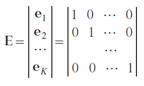
Each vector ek , k = 1,..., K, is the pattern response for class k. Now matrix Y can be represented as a column containing the row vectors yi , i = 1, ... , I.
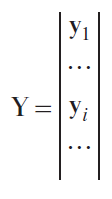
We do not discuss PLS2 regression, as it is explained in many textbooks, e.g., book by Martens and Naes.[24] The data pretreatment is standard: the matrix X is always centred (by columns) and may be scaled depending on the nature of the variables; the matrix Y is only centred. The regression results in the (I × K) matrix of predicted responses Ŷ, which is used as input data for various discriminators, for example, LDA or QDA.
Fig. 4 shows two examples of discrimination that used the same data: the set of near-IR (NIR) spectra recorded for samples of dried oregano (Origanum vulgare): purchased in a store (Store), collected in the wild (Nature), and counterfeit (Fake).[81]
![[{"id":"HTb8unuTqO","type":"paragraph","data":{"text":"Examples of using PLS-DA for deterministic (<i>a</i>) and probabilistic (<i>b</i>) discrimination of oregano (Origanum vulgare) samples: purchased in a store (Store), collected in the wild (Nature), and counterfeit (Fake)"}}]](/storage/images/resized/5nsAbrZ16dy1AEDtYuG7qG5Xu35BwRyV5SAdvtUk_xl.webp)
The left plot (Fig. 4a) shows the result of deterministic discrimination in which the three classes are separated by boundaries.[58] It can be seen that each sample has been assigned to a certain class, in some cases, incorrectly. In the plot on the right (Fig. 4b), the same samples are classified using a probabilistic model, where the decision boundaries depend on the significance level α (in this example, α = 0.1). In this case, there are several samples assigned simultaneously to two classes and there are samples not assigned to any of the classes; therefore, this is a soft classification.
3.2. Authentication using DD-SIMCA
DD-SIMCA is a modern version of the one-class SIMCA method, which is a probabilistic classifier. The decision rule is formulated according to a predefined significance level α, and the distribution parameters are estimated using experimental data. If an alternative class is available, DD-SIMCA provides the possibility of calculating type II error β and construct the corresponding extended decision region, which guarantees that the risk of accepting a sample from the alternative class does not exceed β.
Quite a number of studies are devoted to various aspects of the DD-SIMCA method, and the final description of the method was reported by Kuchertavskiy et al.[82] In brief, the method can be described as a two-stage procedure. In the first stage, like in any sort of SIMCA method, the principal component analysis is applied to the training dataset collected from samples of the target class. The dataset matrix X of size (I × J), centred and/or scaled, is represented in the form:
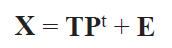
where T = {tia} is the (I × A) matrix of scores; P = {pja} is the loading matrix of size (J × A); E = {eij} is the residual matrix of size (I × J); A is the number of principal components (PCs).
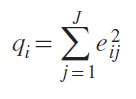
In the second stage, a decision rule is established. The way this rule is chosen determines which variant of the SIMCA method is used.[75] In the DD-SIMCA method, two distances are calculated for each sample of the training set i = 1, ... , I. The first one is orthogonal distance (OD), qi , which is calculated as the squared Euclidean distance from the sample x to the subspace of principal components
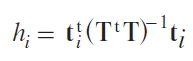
The second one is the score distance (SD), hi , the squared Mahalanobis distance from the model centre to the sample projection in the subspace of principal components
The normalized SD and OD values are described by the chi-square distribution
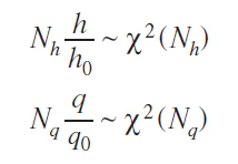
All distribution parameters such as the factors h0 , q0 and the degrees of freedom Nh and Nq are estimated using the corresponding distances calculated for samples of the training set; therefore, the method is called data-driven (DD). The chi-square distribution parameters can be found using either the classical or the robust method. In the absence of outliers, the classical approach provides more accurate results. The robust approach is less sensitive to outliers and, as a result, helps to identify them.[82]
The full distance (FD), f, defined as the weighted sum of h and q, also obeys the chi-square distribution with Nf = Nh + Nq degrees of freedom according to the definition of χ2.
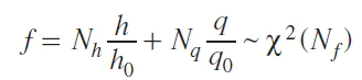
where Nf = Nh + Nq . The full distance is used to establish the critical threshold depending on the significance level α in the following way:
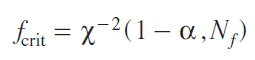
The samples for which the full distance fi satisfies the inequality
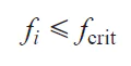
refer to the target class.
Graphically, the classification result can be represented using an acceptance plot in the q/q0 axis against the h/h0 axis (Fig. 5),[83] irrespective of the dimension of the principal component subspace. The green marks (Fig. 5a) designate regular samples of the training set, while the green line indicates the acceptance threshold for the target class.
![[{"id":"6AcOC6WHqe","type":"paragraph","data":{"text":"Examples of using DD-SIMCA. (<i>a</i>) Classification of metronidazole tablets.<sup>83</sup> (<i>b</i>) Determination of tetracycline in blood serum. The result for α = 0.05 (continuous line) and α = 0.15 (dashed line)."}}]](/storage/images/resized/d0HWQhzMa2KW29xsp9TPpGYtvaK7kPZOnmquthcm_xl.webp)
In addition, it is possible to specify the probability γ, which is an appropriate uncertainty in determination of outliers. Then the region of outliers is defined by the boundary

and all training set samples such that

correspond to outliers. The red marks (Fig. 5a) designate outliers among the training set samples; the red line is the outlier boundary. The training set samples located between the acceptance boundary and the outlier boundary (Fig. 5a, yellow marks) are called extremes. If the boundary has been chosen appropriately, the proportion of extremes is close to the significance level α. If samples located within the acceptance region and samples located far beyond the acceptance boundary should be presented in the same plot, a logarithmic axis transformation should be used (Fig. 5b).
If alternative data are available, type II error can be estimated.[84] Let the vector x be a sample from an alternative dataset. If the vector x is projected onto the subspace of principal components based on the target set, the full distance FD for it can be calculated by equations (4) and (5), which use the parameters h0 , q0 , Nh , and Nq found for the target class. Thus, all calculations for the alternative set are similar to those for the target set. The main difference is that the distribution for the alternative set FD is not governed by the standard chi-square distribution, but rather by its generalization: the noncentral chi-square distribution χ' 2(N, s), where N is the number of the degrees of freedom, and s is the noncentrality parameter.
Thus, the type II error (β) can be estimated using the equation
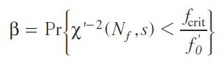
where the fcrit value is defined in equation (8). The noncentrality parameter s and the scaling factor are estimated using the data of the alternative set.[84]
When β is specified, equation (12) can be inverted to find FD corresponding to this error. This method is useful for risk assessments[85] and for determining the limit of detection in one-class classification.
4. Figures of merit
The set of indicators that characterize the quality of a constructed model is collectively referred to as figures of merit and is commonly abbreviated as FoM. We will also use this abbreviation. The concept of FoM encompasses several characteristics: correct sample assignment to particular classes, evaluation of misclassification errors, assessment of model efficiency, and evaluation of the predictive capability of the model.
4.1. Confusion matrix
Irrespective of the classification method, the primary result of classification is the confusion matrix,[86] a table that shows the distribution of predicted samples among the actual classes (Fig. 6). For one-class classification, the confusion matrix is reduced to a single row.
![[{"id":"0iMpxNBHYf","type":"paragraph","data":{"text":"Confusion matrix in the binary classification, K = 2"}}]](/storage/images/resized/7PJJshEWEjQIIQnpVVfyXK2s6SyF8JwnX95MLVZj_xl.webp)
4.2. Binary classification
In the case of binary classification, the size of the confusion matrix is (2 × 2) (see Fig. 6). If the target class is class O, then the elements of the matrix are defined as follows. The TP (true positive) cell shows the number of samples in class O that have been correctly assigned to this class. The FN (false negative) cell presents the number of class O samples that have been erroneously assigned to class C and, hence, they were falsely rejected. The FP (false positive) cell shows the number of samples of class C that have been erroneously assigned to O. Finally, in the TN (true negative) cell, there is the number of samples of class C assigned to class C and, hence, correctly rejected as not belonging to class O. In the binary classification, classes O and C are equivalent; that is, class C can be defined the target class, instead of O; in this case, the true positives and true negatives would exchange places.
The confusion matrix is used to calculate the basic FoMs.[6] They include sensitivity (SNS), which is the proportion or percentage of samples in the target class that are correctly assigned to this class, and specificity (SPC), which is the proportion or percentage of samples from another class that were correctly identified as not belonging to the target class. In the case of hard classification, where each sample necessarily belongs to one of the specified classes, SNS and SPC values are calculated by conventional equations:[86]
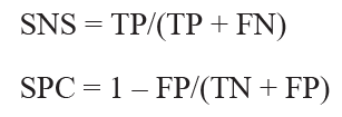
In addition, TP + FN = IO (the number of samples in class O) and TN + FP = IC (the number of samples in class C).
The main drawback of the hard classification is the absence of options such as ‘the sample does not belong to any class at all’, or ‘the sample simultaneously belongs to several classes’. These options are possible only in the soft classification. Meanwhile, in practice, this is quite often the case. For example, a new sample may belong to neither of these two classes (O or C), but rather to a third class Z that was not taken into account in the modelling.[68] In addition, in biomedical problems, there is often no clear boundary between classes.[31][81]
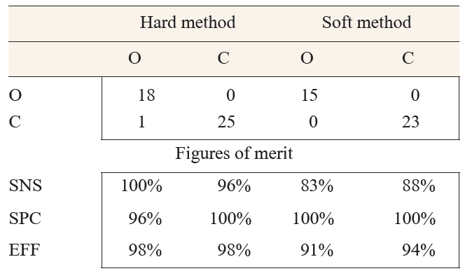
Fig. 7 shows the results of binary discrimination using hard and soft methods. Samples of Brazilian coffee grown by either organic or conventional method were studied. The model was built using 18 samples grown using organic methods (class O) and 26 samples grown using conventional methods (class C). A set of 22 parameters reflecting the composition, physicochemical properties, and antioxidant activity was used as variables.[87]
![[{"id":"CVnhQYzstv","type":"paragraph","data":{"text":"Hard and soft discrimination of Brazilian coffee in terms of the growth methods: organic (O) and conventional (C) techniques"}}]](/storage/images/resized/MPKGxVcKAliBGw0BWVUzHwcVvFWJ96Ve7kXAPwq6_xl.webp)
In Fig. 7, hard discrimination divides the plane into two parts along a vertical black line: O is on the left and C is on the right. It is clear that all samples are reliably discriminated, except for one sample of class C. Soft discrimination is specified by two areas: pink (O) and blue (C). These areas were generated using soft PLS-DA[58] for the significance level α = 0.1. In this case, two samples from class C and three samples from class O remain unclassified, which is reflected in the corresponding confusion matrix (the upper part of Table 1). Here, the same principle as in Fig. 6 is used: the rows correspond to the known class and the columns correspond to the obtained class.
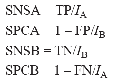
This example shows that in the case of soft classification, equations (13) are inapplicable for calculating sensitivity and specificity, since the total number of samples in each class is not equal to the sum of true positives and false negatives. Therefore, for the general case of discrimination between classes A and B, equations (13) must be written as
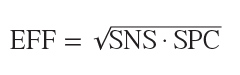
It is useful to introduce another figure of merit that combines the sensitivity and specificity. This is efficiency, which is calculated as the geometric mean, or proportional mean, which allows using this value even when the number of samples in different classes is unbalanced.
All these values are given in the lower part of Table 1.
Apart from the efficiency, another frequently used parameter is accuracy (ACC), which is calculated as the proportion of correctly classified samples divided by the total number of samples

The ACC index works best when the sample sizes for both classes are balanced. For unbalanced classes, in addition to equation (15), the F1-score is also used; it is particularly popular in biomedical research. In addition to the primary figures of merit, there are numerous secondary metrics and indices that characterize the results of classification. For example, Ferri et al.[88] analyzed 18 such metrics, while Sokolova and Lapalme[89] considered 24 metrics. All of these indices and characteristics are combinations of key values of the confusion matrix.
4.3. Multi-class classification
A general classification problem considers I samples representing K target classes with sizes I1 + I2 + ... + IK = I. The classification results can be presented as a confusion matrix of size (K × K). The matrix elements pkl are the numbers of samples of class k assigned to class l. In the case of multi-class classification, the issues related to definition of FoMs have not yet been fully studied,[29][90] with the definitions being more complex. The TP(k) and FP(k) values are defined for each class on the basis of the confusion matrix[91]
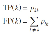
and the appropriate FoMs are calculated separately for each class k
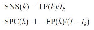
Thus, 2 K indices are collected, and in order to characterize the results of the multi-class model as a whole, Pomerantsev and Rodionova[91] proposed calculating the total figures using the following equations. The total sensitivity (TSNS) was defined as
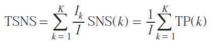
and the total specificity (TSPC) was defined in the following way:

Formulas (18) – (20) are valid for both hard and soft classification methods. The total efficiency TEFF

characterizes the classification model as a whole and serves both for model optimization and for comparison of various models
4.4. One-class classification
In the case of one-class classification, there is only one target class, and all values are calculated relative to that class. As for the alternative (non-target) class, it may be absent; then it is impossible to calculate SPC, and EEF = SNS. Also, there may be several alternative classes. In this case, the specificity should be calculated separately for each of the alternative classes. When the constructed model is applied to new, unknown samples, it makes sense to evaluate only SPC, since there is no information on whether the samples belong to the target class, while the efficiency for a new set, in the absence of class assignment data, is calculated as EFF = SPC.
4.5. A priori characteristics of classification methods
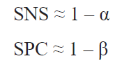
In the description of classification models, it is necessary to distinguish two different sorts of indices. The first one includes, e.g., type I error (α) and type II error (β), which have been borrowed from statistics. In analytical chemistry, they correspond to the sensitivity and specificity. The main difference between the statistical and analytical approaches is that the parameters α and β are specified a priori or calculated theoretically, whereas SNS and SPC are calculated a posteriori, after the model has been built. Type I error α is the significance level, that is, the probability of incorrect rejection of samples of the target class, while β is the probability of incorrect acceptance of samples of other classes as belonging to the target class.[92] For a specified α value, a classifier is developed, and the classification result is evaluated using SNS. If SNS is close to 1 – α, the goal has been achieved, and the model is optimal. Otherwise, the classifier should be adjusted, e.g., by increasing or decreasing the model complexity. The SPC is an a posteriori evaluation of the 1 – β value; therefore, for a well-trained model, one can expect that
Apart from above FoMs, there are other FoMs, e.g., the selectivity and the limit of detection. They are actively used in quantitative analysis, but in qualitative analysis, their definitions and calculation methods were unknown until recently. These issues are discussed in separate parts of the review.
5. Optimization and validation
The optimization and validation of a model are, in essence, the same procedure carried out using the same tools but with different objectives. The procedure includes comparison of the figures of merit (FoMs) achieved upon calibration using the training set with those obtained in the prediction using the independent test set. Optimization is selection of the model parameters that ensure the best performance and robustness. Validation is verification of the fact that the model provides the expected results when used in practice. Each of these procedures requires its own test set.
5.1. Optimization
All classification models used in qualitative analysis have parameters that can be adjusted to improve the model performance. The number of these parameters varies greatly, ranging from one, as in the kNN method, to almost infinity, as in DL methods. In the case of projection methods, this parameter is the dimensionality of the projection space, for example, the number of principal components or latent variables. For algorithms based on the support vectors, these are the regularization parameter and the choice of kernel function; for methods based on search trees, these parameters include the number of trees, the maximum depth, minimum number of samples in a node, and the number of features for splitting. This choice is well formalized[93] in quantitative analysis for the solution of calibration problems. The root-mean-square-errors RMSEC and RMSEP are plotted vs. a complexity parameter (e.g., the number of principal components) and, after that, the point in which RMSEP is minimum is chosen.
Pomerantsev and Rodionova[91] proposed a similar approach for classification using the total efficiency of training (calibration), TEFFC, instead of the error of calibration, RMSEC, and the total efficiency of validation (prediction), TEFFP, instead of the error of prediction, RMSEP. Generally, as the model becomes more complex, the TEFFC first increases and then remains stable. Simultaneously, TEFFP first increases and then decreases. The point of convergence of these two characteristics is chosen as the optimal value for the complexity parameter. In the above example of binary classification of Brazilian coffee (see Fig. 7), there are two possible options. The first one is to choose the number of PLS latent variables, LV = 1; then TEEFC = 90% and TEFFP = 95%, which is a quite reasonable result considering the problem in question. The other option is LV = 3, then TEEFC = 97% and TEFFP = 95% (Fig. 8).
![[{"id":"YifCcBRMbp","type":"paragraph","data":{"text":"Optimization in the binary discrimination of Brazilian coffee: relationship between overall efficiency and model complexity"}}]](/storage/images/resized/VpYLqt2fsEGxxkcdLtPj9g1smREDQqPaHU7guhIA_xl.webp)
As the model complexity further increases, the efficiency on the test set declines, indicating that the classifier is overfitted. The selection of a smaller number of latent variables gives a more robust model, while the dimensionality equal to three reveals a greater difference between the classes. For multi-class classification, the optimization method remains the same, and the total efficiency is calculated using equations (19), (20), (21).
To optimize the deterministic PLS-DA model, it is necessary to find the unique free parameter: the number of latent variables. The probabilistic classifiers have one more parameter, significance level α, which can also be adjusted. The goal of this optimization is to balance the SNS and SPC values by making them approximately equal. This can be done by an approach based on analysis of receiver operating characteristic (ROC) curves.
In the traditional binary classification, the ROC curve characterizes the model performance in the SNS vs. 1 – SPC coordinates and can be used to select the optimal threshold.[76]A convenient ROC approach for multi-class classification has not yet been developed.[94][95]
However, for the probabilistic discriminator PLS-DA presented in Section 3.1, the ROC curve can be constructed in the (1 – TSPC; TSNS) coordinate system by varying the value of α. This curve is shown in Fig. 9. When α = 0, then TSPC = 0 and TSNS = 1, while in the case of α = 1, TSPC = 1 and TSNS = 0. The ‘distance to (0, 1)’ curve is calculated as the distance from the ROC curve to the point with the (0, 1) coordinates. The optimal α value, i.e., the threshold between the classes, is chosen for the minimum value of this distance. The other way for selecting the α value is to plot TEFF as a function of α. The highest point in this curve corresponds to the optimal value of α. Both methods appear to be equivalent, but the former one provides an additional characteristic called ‘area under the curve’ (AUC), that is, the area confined by the ROC curve and the horizontal axis. The higher the AUC value, the better the classifier. In the example shown in Fig. 9, AUC = 0.94, which is a good result.
![[{"id":"iVTEWPctH1","type":"paragraph","data":{"text":"ROC curve for the optimization of the parameter α in the probabilistic model for discrimination of oregano samples"}}]](/storage/images/resized/ftP9vGUrVY3ghtetKenX30D8WeLEym6emrzcy8LK_xl.webp)
5.2. Validation
The validation[96] is a necessary step in the construction of the final model based on formal modelling. The model should be tested using an independent test set, which (1) should not be involved in training of the model; (2) should not be a copy of the training set, e.g., should not consist of repeated measurements of the training set; and (3) should be, as much as possible, a representative selection of samples that would be encountered in the practical use of the model. In an ideal study, it is preferable to use three data sets that represent the population of samples: a training set for model construction, test set No. 1 to optimize the model, and test set No 2 for validation (validation set). Often, a researcher does not have this large number of samples[97] due to various reasons. In this case, two sets are used: a training set and a test set. The test set is selected among the total initial data set either randomly or using various algorithms, such as the Kennard – Stone method, D-optimal design, and others.[98-100] A new approach[101] to the choice of an optimal subset is described in Section 6.6.
Another way to generate a test set is to simulate a new set using statistical modelling. The most popular method is the cross-validation procedure. The most frequently used versatile cross-validation procedures and evaluation of their efficiency in various scenarios were described in detail by Bro et al.[102] In the field of machine learning, the cross-validation procedure has become the gold standard for the model optimization stage.[103]
A double (or nested) cross-validation procedure uses two nested cross-validation loops, which simultaneously evaluate both the model complexity, i.e., optimization step, and the prediction efficiency.[104] However, in some situations, cross-validation is inapplicable. For example, this is the case where data are grouped or contain the results of repeated experiments; or data reflect a process that varies over time; or data have been collected using design of experiments; or a very small data set is used and, hence, every sample is critically important. Therefore, a new method called Procrustes cross-validation (PCV) was recently proposed for generating a simulated set.[105] The method is based on the k-fold cross-validation algorithm; however, unlike the conventional algorithm, the proposed method allows the generation of a new dataset that carries a correct variability evaluated by the cross-validation procedure. This dataset, known as a pseudo-validation (PV) set, can be used in the same way as an independent test set. It can serve to calculate residual distances, explained variance, scores, and other results that cannot be found by conventional cross-validation. This approach makes it possible to model and test small datasets.[106]
5.3. Rigorous and compliant approaches to one-class models
A one-class classifier (OCC) is always based on one (target) class, while other (alternative) classes are ignored in the model. Hence, we cannot calculate SPC, and EFF = SNS. Correspondingly, the number of principal components is optimized by comparing the sensitivity of calibration (SNSC) with the sensitivity of prediction (SNSP). This approach to modelling is called rigorous.[30] Its main advantage is that it is completely independent and can be applied to any alternative classes. However, an analytical chemist often focuses on only one alternative class and seeks to improve the classification quality specifically for this alternative. Then it is possible to calculate the specificity SPC and optimize the number of principal components by comparing EFFC with EFFP. Furthermore, the significance level α can also be optimized using the ROC method described above.[76]This approach is called compliant.[30]
Thus, the benefits of the rigorous approach include the possibility of authentication and versatility, while its drawback is low specificity. For the compliant approach, the opposite is true: the benefit is high specificity, while the drawback is the lack of possibility of authentication, since in this case, OCC simply becomes a discriminator that is not suited for classifying samples of new classes.[68] Note that compliant SIMCA is a poor discriminator compared to PLS-DA.
There is also an intermediate approach that can be called risk management.[85] In this case, several alternative classes are considered, and compliant OCC is formed to maximize the specificity values for all of these classes. This is done by choosing the α value that would minimize type II errors, β, that is, the risk of accepting an alien sample.
6. Cumulative analytical signal
An analytical signal is an important concept in chemistry, which currently lacks a universal definition. In quantitative analysis, an analytical signal is a part of the data that contains information about the substance of interest (analyte). There is no equivalent definition for qualitative analysis. This Section discusses how it can be defined and why it is needed.
6.1. Analytical signal in qualitative analysis
In the simple case of univariate calibration, an analytical signal is understood as a numerical value such as peak height or area under the peak that correlates with the analyte concentration.[107] Multivariate calibration introduces the analytical signal as a mathematical abstraction that represents a combination of regression coefficients. This quantity is called net analytical signal (NAS), that is, the signal that remains after the influence of other components has been eliminated.[108] This is a number or a vector calculated for each calibration sample as an implicit function of a dataset (X, Y) and the regression model used for calibration.
An analytical signal is a condensed expression of the relationship between the concentration of interest and the available experimental data. It is convenient for estimating the selectivity and uncertainty and for determining the limits of detection. Therefore, NAS has numerous applications, such as calculation of FoMs, selection of significant variables, detection of outliers, and model optimization.[109] In qualitative analysis, there is no simple objective such as concentration; instead, there are decisions that are difficult to formalize, e.g., YES/NO/UNKNOWN, the relation of which to data properties (peak height and peak area) is not obvious. However, if we take a closer look at the essence of the classification methods used to make these decisions, we can see that a key role is played by distances. The distances determine the structure and interaction of classes; therefore, in qualitative analysis, we must switch from the ‘more/less’ to ‘closer/further’ indicators.
Three distances are used in analytical chemistry. The first one is the orthogonal distance (OD), q, a common Euclidean metric, that is, the sum of the squares of the coordinates, defined above in equation (4). It is used universally to assess the approximation error,[24] to verify the similarity of spectra,[34] and to address more challenging problems.[39]
The second one is the score distance (SD), h, the squared Mahalanobis distance, which is defined by equation (5). It is used to evaluate the positions of objects for low-dimensional data, so-called features, which appear upon the use of PCA or PLS. It is encountered in many classification methods such as SIMCA, UNEQ, QDA, and so on.
Finally, the third one is the Y-distance (YD) for calibration errors, z:
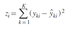
It is used to detect outliers during calibration.[110]
These three distances form the construction kit for the assembly of cumulative analytical signals (CAS). Each of them is a random variable that obeys the chi-square distribution up to parameters that can be estimated using standard statistical methods. In some cases, it is necessary to use the noncentral chi-square distribution, χ' 2(N, s), which includes the noncentrality parameter, s, and a scaling factor. Elementary CAS are non-negative random variables with the additivity property: χ2(N1) + χ2(N2) = χ2(N1 + N2). Therefore, they can be combined, and the result will also follow the chi-square distribution. In addition, they are often independent; therefore, the number of degrees of freedom can simply be added together. That is why this analytical signal is called ‘cumulative’.
In the DD-SIMCA method, a single value, particularly the full distance FD defined in equation (7), can be assigned to each sample (multivariate ‘fingerprint’). This value characterizes the proximity or remoteness of the target sample from the acceptance boundary through equations (8) and (9). Therefore, FD is an example of CAS.
We will consider a few examples of application of the CAS concept that demonstrate its practical significance.
6.2. Limit of detection
The CAS concept makes it possible to develop a new method for calculating the limit of detection for the DD-SIMCA classifier. The main advantage of the CAS approach over existing methods is that it is based on a distribution that is known up to parameters. This opens up the way to simplify the calculation of necessary statistical parameters, such as type I and type II errors, confidence intervals, critical levels, etc. Indeed, if the distribution is unknown, then, for example, to estimate the 0.95 quantile, the sample size must be at least 10 times larger than that in the case of a known parametric distribution. In authentication problems addressed using one-class methods, determination of the limits of detection is often irrelevant, since adulteration of many food products such as vegetable oils,[111-113] honey,[114][115] coffee,[116] and spices[117] by low-concentration adulterants is not economically reasonable. However, the adulteration of essential food products and medicines[21][118][119] requires determination of detection limits, since even low concentrations of impurities can pose a health risk, for example, the addition of ammonium chloride and melamine to milk[120] or the contamination of a propylene glycol-based children syrup with diethylene glycol.[121] Pomerantsev et al.[122] described in detail an algorithm for the calculation of the limit of detection within a one-class classification problem and gave examples of determination of the limits of detection for talc in wheat flour and tetracycline in blood serum.
Determination of tetracycline in blood serum using synchronous fluorescence spectra was first described in detail by Goicoechea and Olivieri[123] and was subsequently used as an example for calculating the detection limits in calibration[124] and qualitative analysis.[122] The classification problem is addressed by forming a target class consisting of 14 pure blood serum samples free of tetracycline contamination. Of these, ten samples were used to train the model and four samples were employed for testing. Four sets (four samples each) consisted of samples contaminated with tetracycline in increasing concentrations of 0.2, 0.4, 0.6, and 0.8 μg mL–1. They were used as the alternative sets. All samples used in the study are depicted in Fig. 5b. The position of each sample indicates its proximity to the acceptance region. Training set samples (open squares) are used to build a model and estimate the boundary of the target class. Test set samples are used to verify that the class boundary was correctly established. All other samples belong to alternative sets. If the threshold is set at a significance level of α = 0.05, then half of the samples with a low tetracycline concentration of 0.2 μg mL–1 are incorrectly identified as being pure. All other alternative classes are well separated, with samples for each particular concentration being grouped together and distinguished from samples of other classes. This example shows that in the presence of several alternative classes, it is advisable to calculate specificity separately for each alternative class. The total specificity for the whole set of tetracycline-containing samples SPC = 87.5%, for the set with concentration of 0.2 μg mL–1, SPC = 50%, and for any other alternative sets containing ≥0.4 μg mL–1 of tetracycline, SPC = 100%.
According to a definition,[125] the limit of detection (LOD) is the minimum amount of the analyte that can be distinguished from the blank with specified probabilities of type I (α) and type II (β) errors. The former error (α) is the probability that the analyte is detected in the sample, while in reality, this sample is blank. This error is characterized by the decision threshold (CCα), that is, the CAS value corresponding to the critical level. Type II error (β) is the probability that a sample is reported as negative, while the analyte is actually present. This error is characterized by the limit of detection (CCβ), i.e., the lowest content of analyte that can be detected in the sample with the probability β. To avoid confusion, it is important to emphasize that CCα is expressed in the same units as CAS (most often, dimensionless), whereas CCβ is expressed in analyte concentration units.
Fig. 10a illustrates the calculation of two limits of detection for α = 0.01, which corresponds to CCα = 23. The minimum concentration at which tetracycline can be detected is CCmin = 0.21 μg mL–1; however, the probability of error in this case is high and equals 0.95. The maximum concentration at which tetracycline can be detected in blood serum with a low probability of error of 0.05 is CCmax = 0.30 μg mL–1. The curves (blue and red lines) were plotted using equation (12) inverted to find FD (β).
![[{"id":"gyfdoh0CD_","type":"paragraph","data":{"text":"Determination of tetracycline in blood serum: (<i>a</i>) calculation of the limit of detection; (<i>b</i>) selectivity curves for two alternative classes"}}]](/storage/images/resized/SiSR6GqV7bO3c8nRZkdbgaVHU6qRgc55qESrG87p_xl.webp)
6.3. Selectivity
Qualitative analysis always includes three main elements: the object, the method, and the tool. The object is a part of reality that is being studied. For example, this can be melamine in powdered milk, which must be detected, or a medication that must be tested for authenticity. The method means the analytical platform used to gain data about the object: spectroscopy, chromatography, etc. Finally, the term ‘tool’ refers to the mathematical procedure used to analyze data and make decisions.
Each element of this triad can be compared to an analogue, provided that the other two elements are identical. For example, it can be stated that NIR spectroscopy is more effective than UV-visible spectroscopy for detecting talc in flour, or that a one-class classifier is more suitable for authentication than a discriminator. This brings us to the concept of selectivity (SLС), which is used to compare objects, methods, and tools and which is considered to be important by many analytical chemists.
It is not entirely clear how to define SLC in qualitative analysis. Only two facts are known for certain: (1) SLC is a limiting case of SPC[126] and (2) selectivity is the ability to minimize false positive results.[127]
In the DD-SIMCA method, the probability of false positive results is expressed in terms of type II error (β), which is calculated as described by Pomerantsev and Rodionova.[84] Thus, in the context of qualitative analysis, the following definition of selectivity is proposed. Selectivity is the expected probability of true negative results:[128]
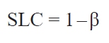
It is important to find the right place for SLC among other figures of merit. SNS and SPC are empirical characteristics determined by counting the number of true positive and true negative decisions; therefore, they are subject to errors. Another pair consists of the probabilities α and β, one being set a priori (most often, α) and the other being calculated theoretically. SPC is an empirical estimate of the probability that the analytical process correctly classifies a non-target sample as not belonging to the target class. SLC is the theoretically expected limiting value of SPC that can be achieved in an ideal experiment in which the sampling variability is negligibly small or the sampling size is very large.
Consider how this works for the tetracycline example. If the value of α is changed to α = 0.15 (the dashed line in the plot, Fig. 5b), then all samples containing tetracycline will be correctly classified as not belonging to the target class, i.e., SPC = 100% for each alternative class. However, it is clear that the 0.2 μg mL–1 class is located much closer to the acceptance region than the 0.4 μg mL–1 class and, all the more, closer than other alternative samples. In this case, for the class of 0.2 μg mL–1, SLC = 93%, since β = 0.07, while for the class of 0.4 μg mL–1, SLC = 100% and β = 7 × 10–17.
Since SLC depends on the chosen value of α, it is useful to represent it as the curve shown in Fig. 10b. This curve resembles the ROC curve. The area under this curve (AUC) can be used as an integral measure of selectivity. For example, for the 0.2 μg mL–1 class, AUC = 94%, while for the 0.4 μg mL–1 class, AUC = 100%; hence, the latter class is more selective.
The selectivity can be applied at various stages of qualitative analysis. First, to compare different datasets, for example, to determine which of the alternative sets is closer to the target class (Fig. 10b). Second, the selectivity helps to understand which instrumental method has higher selectivity when applied to the same set of samples (Fig. 11a). Third, the selectivity, especially in its integral form, allows for the comparison of data analysis tools[129] (Fig. 11b).
![[{"id":"lCk0ev2yN-","type":"paragraph","data":{"text":"Authentication of olive oil. (<i>a</i>) Selectivity of various instrumental methods: M1, M2, ... , M4. (<i>b</i>) Changes in the selectivity upon successive fusion of the data blocks obtained using different tools: M1, M1 + M2, ... , M1 + M2 + M3 + M4."}}]](/storage/images/resized/Dfil9z3PKiQzP8KwhiHbY0obF47tlEpYRE6Ong5w_xl.webp)
6.4. Detection of outliers
A modern approach to outlier detection is based on the philosophy of machine learning. It includes the simultaneous use of various outlier detection techniques.[130][131] An example is a general-purpose tool that uses the sum of ranking differences,[132] which is sensitive to various types of outliers and requires significant computational resources.
Rodionova and Pomerantsev[110] proposed a simple approach to outlier detection that was called sequential focused trimming. For this purpose, the total distance TD (Total Distance), g, is used, which is a CAS composed of three basic elements:
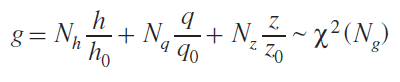
where Ng = Nh + Nq + Nz . For the chosen significance level γ (an admissible false positive error), the decision rule is specified by the following condition:
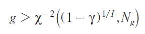
where I is the number of samples in the dataset.
The procedure starts with a model that uses the entire training set. This serves to estimate all three basic elements of CAS: q (OD), h (SD), and z (YD) [equations (4), (5), and (23)] and to calculate CAS g (TD). Unlike the conventional approach, which uses two separate cut-off thresholds for the X and Y residuals, the method based on CAS calculates a joint critical area. The advantages of this approach are as follows:[82] (1) all distribution parameters are calculated from the data; therefore, this is a data driven approach; (2) both classical and robust methods are used to estimate the parameters; (3) the probability γ used to calculate the boundary for the outlier region is specified a priori and has a statistical meaning; (4) the detected outliers are eliminated sequentially, one by one, which makes it possible to avoid the masking and swamping effects.
6.5. Data fusion
Data fusion methods are used for joint analysis of the data obtained using various analytical platforms for the same samples.[133] In this context, three levels of fusion are distinguished. The first one, also called low, involves merging of the results of measurements (blocks) obtained using various instruments into a single data block, which is then utilized to build a single common model. According to the mid-level fusion, each block is separately processed to extract information; for example, principal components that are identified using the PCA method, variables that are selected, and so on. After that, the features identified for each block are combined into a common predictor matrix for which the model is built.[134]
High-level fusion is performed by combining the modelling results for each data block. In practice, these methods are rarely encountered, as they are more complex than first- and second-level methods.[135] The use of the CAS-based approach makes high-level fusion simple and straightforward, since it is based on combining the single CAS values obtained by modelling separate data blocks. Any number of diverse blocks can be combined in this way. Although high-level fusion finally results in a fairly complex model, analysis of partial FD distances for each of the blocks makes it possible to establish a significant relationship between the classification results and the effect of particular samples and instruments. For example, the possibility of authentication of olive oil samples was investigated both using particular instruments (Fourier transform NIR spectroscopy, UV spectroscopy, electronic tongue, and electronic nose) and using joint classification incorporating all four analytical methods.[136] The result shown in Fig. 11 illustrates the benefits of data fusion.
Lozano et al.[129] used CAS-based approach for fusing a three-dimensional tensor of fluorescence data and a two-dimensional matrix of spectral data.
6.6. Selection of sample subset
Analysis of large datasets faces the challenge of selecting a subset of samples that meets particular criteria from the whole original dataset. This problem can be split into two tasks.[101] The first one is the choice of a reduced dataset that does not compromise the prediction accuracy, but is markedly smaller than the original dataset. This subset is typically used for calibration transfer[137] or for image analysis.[138] The second one is the selection of the test set. On the one hand, the test set should reflect the variability of the target class as fully as possible; on the other hand, it should differ from the training set. Typically, the test set comprises 25 – 30% of the total dataset and is used to optimize and validate the model.[97][139] The CAS concept can be used for effective selection of these subsets for both single-block (classification) and multi-block (calibration) data. As a result of simple calculations, sample importance (SI) index based on the full distance FD is assigned to each sample in the total dataset. The sample importance index takes values in the (0, 1) range, with the higher values corresponding to more important samples. This allows for a targeted, rather than random, selection of samples with specified properties. Samples with the maximum SI values are selected for the reduced set. In the formation of the test set, samples with the minimum and maximum SI values are excluded, and then a specified proportion is selected at random from the remaining samples. It was shown that the proposed method is more efficient than the Kennard – Stone algorithm[98] or D-optimal planning.[99] In addition, it was shown[140] that the importance index slightly depends on the model complexity, which breaks the vicious cycle in which the representative sampling depends on the model complexity, while the model complexity is tested against the representative sampling.
7. Prospects
It is always difficult to make predictions, especially about the future, but we will try. Previously, it was noted that every analytical procedure includes three components: object of the study, instrumental method, and data analysis tool. We will state our ideas on the prospects of qualitative analysis in terms of this structure.
7.1. Objects
Currently, qualitative analysis has been widely and successfully applied to study food products,[141][142] animal feed,[143] pharmaceuticals,[144] and the environment;[145] however, more important and complex objects related to medicine[146][147] and biology[148] are now on the horizon. First of all, this is diagnosis and personalized therapy.[149] Here, the focus is on the qualitative classification of disease stages and types and selection of therapy based on the patient’s personal data.[150] In this field, qualitative analysis is difficult to perform for one reason, which can be summed up simply as human factor. First, the subjects themselves, which are patients, differ from one another much more appreciably than, e.g., samples of oil or tablets, which means higher variability with inevitable extremes and outliers. Second, there are no reliable reference methods, and all model training relies on the subjective opinions of experts, who are prone to mistakes.
7.2. Methods (instruments)
Here, two trends can be distinguished. The first one is the miniaturization of instruments. The fact that NIR spectrometers can be pocket-size devices is no longer surprising to anyone, but portable mass spectrometers[151] and even NMR spectrometers[152] are also appearing. Certainly, they are inferior to their desktop analogues, but they open up new opportunities for conducting qualitative analysis in the field.
The second trend is called point of care (POC):[153][154] this is medical diagnosis performed directly at the patient location in a clinic, in a pharmacy, or at home. This approach provides quick results without the need for specialized laboratories. This is done using compact devices and soft sensors,[155-158] which differ radically from the simple sensors used to detect target substances. This field is experiencing a real boom: suffice is to say that in just four months of 2026, 136 papers on POC were published in Microchemical J. alone, one of the publications being from Russia.[159]
7.3. Data analysis tools
Everything that is now happening in the world and will continue to happen for some time in the future is concentrated on artificial intelligence (AI). This term is misleading, but it has already become deeply ingrained in the consciousness of the general public, including scientists. This term is used, most often, to mean large language models (LLMs), that is, ANNs trained on huge datasets to understand and generate texts. They are good at tasks such as translation and abstracting. Examples are GPT-4, Claude, etc.
It is believed that AI can serve as a useful tool, especially in the field of image analysis. However, this does not mean that it should replace human decision makers, since recognition requires taking into account a multitude of additional factors that constitute domain knowledge.[160] Integration of the domain knowledge could bridge the gap between data analysis and decision making.[161][162]
In our opinion, this integration should be carried out at two levels. At the first basic level, the ML model is adapted to take account of the key characteristics of the domain, constraints, logical rules, etc. The second level is more complex, since it aims to take into account the human factor. This is achieved through collaboration between a group of subject matter experts and a group of data analysts, meant to address any shortcomings resulting from the decisions made by each group. The process begins with data collection, continues through the exploratory analysis phase, and concludes with the decision making stage.
8. List of abbreviations and symbols
This following abbreviations and symbols are used in the review:
α — significance level for acceptance,
γ — significance level of outlier,
χ' 2 — noncentral chi-square distribution,
χ–2 — quantile of the chi-square distribution,
AI — artificial intelligence,
ANN — artificial neural networks,
AUC — area under curve,
CAS — cumulative analytical signal,
DD-SIMCA — data driven SIMCA,
DL — deep learning,
EFF — efficiency,
FD — full distance,
FoM — figures of merit,
FN — false negative,
FP — false positive,
I — number of samples,
IUPAC — International Union of Pure and Applied Chemistry,
J — number of variables,
K — number of classes,
kNN — k-nearest neighbours,
LDA — linear discriminant analysis,
LOD — limit of detection,
LV — latent variables,
ML — machine learning,
N — number of degrees of freedom,
NAS — net analytical signal,
OCC — one class classifier,
OC-PLS — one class PLS,
OC-RF — one-class random forest,
OD — orthogonal distance,
P — loading matrix,
PCA — principal component analysis,
PCR — principal component regression,
PCV — Procrustes cross-validation,
PLS — partial least squares,
PLS-DA — PLS discriminant analysis,
POC — point of care,
PV set — pseudo validation set,
QDA — quadratic discriminant analysis,
RF — random forest,
RMSE — root mean squared error,
ROC — receiver operating characteristic,
SD — score distance,
SEL — selectivity,
SI — sample importance,
SIMCA — soft independent modelling of class analogy,
SNS — sensitivity,
SPC — specificity,
SVM — support vector machine,
T — score matrix,
TD — total distance,
TEFF — total efficiency,
TN — true negative,
TP — true positive,
TSNS — total sensitivity,
TSPC — total specificity,
UNEQ — unequal class models,
YD — Y-distance.
References